Manipulating Data in R
Recap of Data Cleaning
is.na(),any(is.na()),count(), and functions fromnaniarlikegg_miss_var()can help determine if we haveNAvaluesfilter()automatically removesNAvalues - can’t confirm or deny if condition is met (need| is.na()to keep them)drop_na()can help you removeNAvalues from a variable or an entire data frameNAvalues can change your calculation results- think about what
NAvalues represent
Recap of Data Cleaning
recode()can help with simple recoding (not based on condition but simple swap)case_when()can recode entire values based on conditions- remember
case_when()needsTRUE ~ varaibleto keep values that aren’t specified by conditions, otherwise will beNA
- remember
stringrpackage has great functions for looking for specific parts of values especiallyfilter()andstr_detect()combined- also has other useful string manipulation functions like
str_replace()and more! separate()can split columns into additional columnsunite()can combine columns
- also has other useful string manipulation functions like
- Day 5 Cheatsheet
Manipulating Data
In this module, we will show you how to:
- Reshape data from wide to long
- Reshape data from long to wide
- Merge Data/Joins
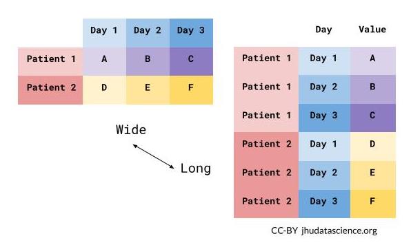
What is wide/long data?
https://github.com/gadenbuie/tidyexplain/blob/main/images/tidyr-pivoting.gif
What is wide/long data?
Data is stored differently in the tibble.
Wide: has many columns
# A tibble: 1 × 4
  State   June_vacc_rate May_vacc_rate April_vacc_rate
  <chr>   <chr>          <chr>         <chr>
1 Alabama 37.2%          36.0%         32.4%
Long: column names become data
# A tibble: 3 × 3
  State   name            value
  <chr>   <chr>           <chr>
1 Alabama June_vacc_rate  37.2%
2 Alabama May_vacc_rate   36.0%
3 Alabama April_vacc_rate 32.4%
What is wide/long data?
Wide: multiple columns per individual, values spread across multiple columns
# A tibble: 2 × 4
  State   June_vacc_rate May_vacc_rate April_vacc_rate
  <chr>   <chr>          <chr>         <chr>
1 Alabama 37.2%          36.0%         32.4%
2 Alaska  47.5%          46.2%         41.7%
Long: multiple rows per observation, a single column contains the values
# A tibble: 6 × 3
  State   name            value
  <chr>   <chr>           <chr>
1 Alabama June_vacc_rate  37.2%
2 Alabama May_vacc_rate   36.0%
3 Alabama April_vacc_rate 32.4%
4 Alaska  June_vacc_rate  47.5%
5 Alaska  May_vacc_rate   46.2%
6 Alaska  April_vacc_rate 41.7%
What is wide/long data?
Data is wide or long with respect to certain variables.
Why do we need to switch between wide/long data?
Wide: Easier for humans to read
# A tibble: 2 × 4
  State   June_vacc_rate May_vacc_rate April_vacc_rate
  <chr>   <chr>          <chr>         <chr>
1 Alabama 37.2%          36.0%         32.4%
2 Alaska  47.5%          46.2%         41.7%
Long: Easier for R to make plots & do analysis
# A tibble: 6 × 3
  State   name            value
  <chr>   <chr>           <chr>
1 Alabama June_vacc_rate  37.2%
2 Alabama May_vacc_rate   36.0%
3 Alabama April_vacc_rate 32.4%
4 Alaska  June_vacc_rate  47.5%
5 Alaska  May_vacc_rate   46.2%
6 Alaska  April_vacc_rate 41.7%
Pivoting using tidyr package
tidyr allows you to “tidy” your data. We will be talking about:
pivot_longer- make multiple columns into variables, (wide to long)pivot_wider- make a variable into multiple columns, (long to wide)separate- string into multiple columns (review)
The reshape command exists. It is a confusing function. Don’t use it.
You might see old functions gather and spread when googling. These are the old names for pivot_longer and pivot_wider, respectively.
pivot_longer…
Reshaping data from wide to long
pivot_longer() - puts column data into rows (tidyr package)
- First describe which columns we want to “pivot_longer”
{long_data} <- {wide_data} %>% pivot_longer(cols = {columns to pivot})Reshaping data from wide to long
wide_data# A tibble: 1 × 3
June_vacc_rate May_vacc_rate April_vacc_rate
<chr> <chr> <chr>
1 37.2% 36.0% 32.4% long_data <- wide_data %>% pivot_longer(cols = everything())
long_data# A tibble: 3 × 2
name value
<chr> <chr>
1 June_vacc_rate 37.2%
2 May_vacc_rate 36.0%
3 April_vacc_rate 32.4%Reshaping data from wide to long
pivot_longer() - puts column data into rows (tidyr package)
- First describe which columns we want to “pivot_longer”
names_to =gives a new name to the pivoted columnsvalues_to =gives a new name to the values that used to be in those columns
{long_data} <- {wide_data} %>% pivot_longer(cols = {columns to pivot},
                                        names_to = {New column name: contains old column names},
                                        values_to = {New column name: contains cell values})
Reshaping data from wide to long
wide_data# A tibble: 1 × 3
June_vacc_rate May_vacc_rate April_vacc_rate
<chr> <chr> <chr>
1 37.2% 36.0% 32.4% long_data <- wide_data %>% pivot_longer(cols = everything(),
names_to = "Month",
values_to = "Rate")
long_data# A tibble: 3 × 2
Month Rate
<chr> <chr>
1 June_vacc_rate 37.2%
2 May_vacc_rate 36.0%
3 April_vacc_rate 32.4%Data used: Charm City Circulator
http://jhudatascience.org/intro_to_r/data/Charm_City_Circulator_Ridership.csv
library(jhur)
circ <- read_circulator()
head(circ, 5)
# A tibble: 5 × 15
day date orang…¹ orang…² orang…³ purpl…⁴ purpl…⁵ purpl…⁶ green…⁷ green…⁸
<chr> <chr> <dbl> <dbl> <dbl> <dbl> <dbl> <dbl> <dbl> <dbl>
1 Monday 01/1… 877 1027 952 NA NA NA NA NA
2 Tuesday 01/1… 777 815 796 NA NA NA NA NA
3 Wednesd… 01/1… 1203 1220 1212. NA NA NA NA NA
4 Thursday 01/1… 1194 1233 1214. NA NA NA NA NA
5 Friday 01/1… 1645 1643 1644 NA NA NA NA NA
# … with 5 more variables: greenAverage <dbl>, bannerBoardings <dbl>,
# bannerAlightings <dbl>, bannerAverage <dbl>, daily <dbl>, and abbreviated
# variable names ¹orangeBoardings, ²orangeAlightings, ³orangeAverage,
# ⁴purpleBoardings, ⁵purpleAlightings, ⁶purpleAverage, ⁷greenBoardings,
# ⁸greenAlightingsReshaping data from wide to long
long <- circ %>%
  pivot_longer(starts_with(c("orange","purple","green","banner")))
long
# A tibble: 13,752 × 5
day date daily name value
<chr> <chr> <dbl> <chr> <dbl>
1 Monday 01/11/2010 952 orangeBoardings 877
2 Monday 01/11/2010 952 orangeAlightings 1027
3 Monday 01/11/2010 952 orangeAverage 952
4 Monday 01/11/2010 952 purpleBoardings NA
5 Monday 01/11/2010 952 purpleAlightings NA
6 Monday 01/11/2010 952 purpleAverage NA
7 Monday 01/11/2010 952 greenBoardings NA
8 Monday 01/11/2010 952 greenAlightings NA
9 Monday 01/11/2010 952 greenAverage NA
10 Monday 01/11/2010 952 bannerBoardings NA
# … with 13,742 more rowsReshaping data from wide to long
There are many ways to select the columns we want. Use ?tidyr_tidy_select to look at more column selection options.
long <- circ %>%
  pivot_longer( !c(day, date, daily))
long
# A tibble: 13,752 × 5
day date daily name value
<chr> <chr> <dbl> <chr> <dbl>
1 Monday 01/11/2010 952 orangeBoardings 877
2 Monday 01/11/2010 952 orangeAlightings 1027
3 Monday 01/11/2010 952 orangeAverage 952
4 Monday 01/11/2010 952 purpleBoardings NA
5 Monday 01/11/2010 952 purpleAlightings NA
6 Monday 01/11/2010 952 purpleAverage NA
7 Monday 01/11/2010 952 greenBoardings NA
8 Monday 01/11/2010 952 greenAlightings NA
9 Monday 01/11/2010 952 greenAverage NA
10 Monday 01/11/2010 952 bannerBoardings NA
# … with 13,742 more rowsReshaping data from wide to long
long %>% count(name)# A tibble: 12 × 2
name n
<chr> <int>
1 bannerAlightings 1146
2 bannerAverage 1146
3 bannerBoardings 1146
4 greenAlightings 1146
5 greenAverage 1146
6 greenBoardings 1146
7 orangeAlightings 1146
8 orangeAverage 1146
9 orangeBoardings 1146
10 purpleAlightings 1146
11 purpleAverage 1146
12 purpleBoardings 1146Cleaning up long data
We will use str_replace from the stringr package to put _ in the names
long <- long %>% mutate(
  name = str_replace(name, "Board", "_Board"),
  name = str_replace(name, "Alight", "_Alight"),
  name = str_replace(name, "Average", "_Average")
)
long
# A tibble: 13,752 × 5
day date daily name value
<chr> <chr> <dbl> <chr> <dbl>
1 Monday 01/11/2010 952 orange_Boardings 877
2 Monday 01/11/2010 952 orange_Alightings 1027
3 Monday 01/11/2010 952 orange_Average 952
4 Monday 01/11/2010 952 purple_Boardings NA
5 Monday 01/11/2010 952 purple_Alightings NA
6 Monday 01/11/2010 952 purple_Average NA
7 Monday 01/11/2010 952 green_Boardings NA
8 Monday 01/11/2010 952 green_Alightings NA
9 Monday 01/11/2010 952 green_Average NA
10 Monday 01/11/2010 952 banner_Boardings NA
# … with 13,742 more rowsCleaning up long data
Now each var is Boardings, Averages, or Alightings. We use “into =” to name the new columns and “sep =” to show where the separation should happen.
long <- long %>%
  separate(name, into = c("line", "type"), sep = "_")
long
# A tibble: 13,752 × 6
day date daily line type value
<chr> <chr> <dbl> <chr> <chr> <dbl>
1 Monday 01/11/2010 952 orange Boardings 877
2 Monday 01/11/2010 952 orange Alightings 1027
3 Monday 01/11/2010 952 orange Average 952
4 Monday 01/11/2010 952 purple Boardings NA
5 Monday 01/11/2010 952 purple Alightings NA
6 Monday 01/11/2010 952 purple Average NA
7 Monday 01/11/2010 952 green Boardings NA
8 Monday 01/11/2010 952 green Alightings NA
9 Monday 01/11/2010 952 green Average NA
10 Monday 01/11/2010 952 banner Boardings NA
# … with 13,742 more rowspivot_wider…
Reshaping data from long to wide
pivot_wider() - spreads row data into columns (tidyr package)
names_from =the old column whose contents will be spread into multiple new column names.values_from =the old column whose contents will fill in the values of those new columns.
{wide_data} <- {long_data} %>%
  pivot_wider(names_from = {Old column name: contains new column names},
              values_from = {Old column name: contains new cell values})
Reshaping data from long to wide
long_data# A tibble: 3 × 2
Month Rate
<chr> <chr>
1 June_vacc_rate 37.2%
2 May_vacc_rate 36.0%
3 April_vacc_rate 32.4%wide_data <- long_data %>% pivot_wider(names_from = "Month",
values_from = "Rate")
wide_data# A tibble: 1 × 3
June_vacc_rate May_vacc_rate April_vacc_rate
<chr> <chr> <chr>
1 37.2% 36.0% 32.4% Reshaping Charm City Circulator
long# A tibble: 13,752 × 6
day date daily line type value
<chr> <chr> <dbl> <chr> <chr> <dbl>
1 Monday 01/11/2010 952 orange Boardings 877
2 Monday 01/11/2010 952 orange Alightings 1027
3 Monday 01/11/2010 952 orange Average 952
4 Monday 01/11/2010 952 purple Boardings NA
5 Monday 01/11/2010 952 purple Alightings NA
6 Monday 01/11/2010 952 purple Average NA
7 Monday 01/11/2010 952 green Boardings NA
8 Monday 01/11/2010 952 green Alightings NA
9 Monday 01/11/2010 952 green Average NA
10 Monday 01/11/2010 952 banner Boardings NA
# … with 13,742 more rowsReshaping Charm City Circulator
wide <- long %>% pivot_wider(names_from = "type",
                             values_from = "value")
wide
# A tibble: 4,584 × 7
day date daily line Boardings Alightings Average
<chr> <chr> <dbl> <chr> <dbl> <dbl> <dbl>
1 Monday 01/11/2010 952 orange 877 1027 952
2 Monday 01/11/2010 952 purple NA NA NA
3 Monday 01/11/2010 952 green NA NA NA
4 Monday 01/11/2010 952 banner NA NA NA
5 Tuesday 01/12/2010 796 orange 777 815 796
6 Tuesday 01/12/2010 796 purple NA NA NA
7 Tuesday 01/12/2010 796 green NA NA NA
8 Tuesday 01/12/2010 796 banner NA NA NA
9 Wednesday 01/13/2010 1212. orange 1203 1220 1212.
10 Wednesday 01/13/2010 1212. purple NA NA NA
# … with 4,574 more rowsSummary
tidyrpackage helps us convert between wide and long datapivot_longer()goes from wide -> long- Specify columns you want to pivot
- Specify
names_to =andvalues_to =for custom naming
pivot_wider()goes from long -> wide- Specify
names_from =andvalues_from =
- Specify
Lab Part 1
💻 Lab
Joining in dplyr
- Merging/joining data sets together - usually on key variables, usually “id”
?join- see different types of joining fordplyrinner_join(x, y)- only rows that match forxandyare keptfull_join(x, y)- all rows ofxandyare keptleft_join(x, y)- all rows ofxare kept even if not merged withyright_join(x, y)- all rows ofyare kept even if not merged withxanti_join(x, y)- all rows fromxnot inykeeping just columns fromx.
Merging: Simple Data
data_As# A tibble: 2 × 3
State June_vacc_rate May_vacc_rate
<chr> <chr> <chr>
1 Alabama 37.2% 36.0%
2 Alaska 47.5% 46.2% data_cold# A tibble: 2 × 2
State April_vacc_rate
<chr> <chr>
1 Maine 32.4%
2 Alaska 41.7% Inner Join
https://github.com/gadenbuie/tidyexplain/blob/main/images/inner-join.gif

Inner Join
ij = inner_join(data_As, data_cold)Joining, by = "State"ij# A tibble: 1 × 4
State June_vacc_rate May_vacc_rate April_vacc_rate
<chr> <chr> <chr> <chr>
1 Alaska 47.5% 46.2% 41.7% Left Join
https://raw.githubusercontent.com/gadenbuie/tidyexplain/main/images/left-join.gif
Left Join
lj = left_join(data_As, data_cold)Joining, by = "State"lj# A tibble: 2 × 4
State June_vacc_rate May_vacc_rate April_vacc_rate
<chr> <chr> <chr> <chr>
1 Alabama 37.2% 36.0% <NA>
2 Alaska 47.5% 46.2% 41.7% Install tidylog package to log outputs
# install.packages("tidylog")
library(tidylog)
left_join(data_As, data_cold)
Joining, by = "State"
left_join: added one column (April_vacc_rate)
> rows only in x 1
> rows only in y (1)
> matched rows 1
> ===
> rows total 2# A tibble: 2 × 4
State June_vacc_rate May_vacc_rate April_vacc_rate
<chr> <chr> <chr> <chr>
1 Alabama 37.2% 36.0% <NA>
2 Alaska 47.5% 46.2% 41.7% Right Join
https://raw.githubusercontent.com/gadenbuie/tidyexplain/main/images/right-join.gif

Right Join
rj <- right_join(data_As, data_cold)Joining, by = "State"
right_join: added one column (April_vacc_rate)
> rows only in x (1)
> rows only in y 1
> matched rows 1
> ===
> rows total 2rj# A tibble: 2 × 4
State June_vacc_rate May_vacc_rate April_vacc_rate
<chr> <chr> <chr> <chr>
1 Alaska 47.5% 46.2% 41.7%
2 Maine <NA> <NA> 32.4% Left Join: Switching arguments
lj2 <- left_join(data_cold, data_As)Joining, by = "State"
left_join: added 2 columns (June_vacc_rate, May_vacc_rate)
> rows only in x 1
> rows only in y (1)
> matched rows 1
> ===
> rows total 2lj2# A tibble: 2 × 4
State April_vacc_rate June_vacc_rate May_vacc_rate
<chr> <chr> <chr> <chr>
1 Maine 32.4% <NA> <NA>
2 Alaska 41.7% 47.5% 46.2% Full Join
https://raw.githubusercontent.com/gadenbuie/tidyexplain/main/images/full-join.gif
Full Join
fj <- full_join(data_As, data_cold)Joining, by = "State"
full_join: added one column (April_vacc_rate)
> rows only in x 1
> rows only in y 1
> matched rows 1
> ===
> rows total 3fj# A tibble: 3 × 4
State June_vacc_rate May_vacc_rate April_vacc_rate
<chr> <chr> <chr> <chr>
1 Alabama 37.2% 36.0% <NA>
2 Alaska 47.5% 46.2% 41.7%
3 Maine <NA> <NA> 32.4% Watch out for “includes duplicates”
data_As# A tibble: 2 × 2
State state_bird
<chr> <chr>
1 Alabama wild turkey
2 Alaska willow ptarmigandata_cold# A tibble: 3 × 3
State vacc_rate month
<chr> <chr> <chr>
1 Maine 32.4% April
2 Alaska 41.7% April
3 Alaska 46.2% May Watch out for “includes duplicates”
lj <- left_join(data_As, data_cold)Joining, by = "State"
left_join: added 2 columns (vacc_rate, month)
> rows only in x 1
> rows only in y (1)
> matched rows 2 (includes duplicates)
> ===
> rows total 3Watch out for “includes duplicates”
Data including the joining column (“State”) has been duplicated.
lj# A tibble: 3 × 4
State state_bird vacc_rate month
<chr> <chr> <chr> <chr>
1 Alabama wild turkey <NA> <NA>
2 Alaska willow ptarmigan 41.7% April
3 Alaska willow ptarmigan 46.2% May Note that “Alaska willow ptarmigan” appears twice.
Watch out for “includes duplicates”
https://github.com/gadenbuie/tidyexplain/blob/main/images/left-join-extra.gif
Stop tidylog
unloadNamespace("tidylog")Duplicated
- The
duplicatedfunction can give you indications if there are duplicates in a vector:
duplicated(1:5)[1] FALSE FALSE FALSE FALSE FALSEduplicated(c(1:5, 1))[1] FALSE FALSE FALSE FALSE FALSE TRUElj %>% mutate(dup_State = duplicated(State))# A tibble: 3 × 5
State state_bird vacc_rate month dup_State
<chr> <chr> <chr> <chr> <lgl>
1 Alabama wild turkey <NA> <NA> FALSE
2 Alaska willow ptarmigan 41.7% April FALSE
3 Alaska willow ptarmigan 46.2% May TRUE Using the by argument
By default joins use the intersection of column names. If by is specified, it uses that.
full_join(data_As, data_cold, by = "State")# A tibble: 4 × 4
State state_bird vacc_rate month
<chr> <chr> <chr> <chr>
1 Alabama wild turkey <NA> <NA>
2 Alaska willow ptarmigan 41.7% April
3 Alaska willow ptarmigan 46.2% May
4 Maine <NA> 32.4% AprilUsing the by argument
You can join based on multiple columns by using something like by = c(col1, col2).
If the datasets have two different names for the same data, use:
full_join(x, y, by = c("a" = "b"))Using “setdiff”
We might want to determine what indexes ARE in the first dataset that AREN’T in the second:
data_As# A tibble: 2 × 2
State state_bird
<chr> <chr>
1 Alabama wild turkey
2 Alaska willow ptarmigandata_cold# A tibble: 3 × 3
State vacc_rate month
<chr> <chr> <chr>
1 Maine 32.4% April
2 Alaska 41.7% April
3 Alaska 46.2% May Using “setdiff”
Use setdiff to determine what indexes ARE in the first dataset that AREN’T in the second:
A_states <- data_As %>% pull(State)
cold_states <- data_cold %>% pull(State)setdiff(A_states, cold_states)[1] "Alabama"setdiff(cold_states, A_states)[1] "Maine"Summary
- Merging/joining data sets together - assumes all column names that overlap
- use the
by = c("a" = "b")if they differ
- use the
inner_join(x, y)- only rows that match forxandyare keptfull_join(x, y)- all rows ofxandyare keptleft_join(x, y)- all rows ofxare kept even if not merged withyright_join(x, y)- all rows ofyare kept even if not merged withx- Use the
tidylogpackage for a detailed summary setdiff(x, y)shows what inxis missing fromy
Lab Part 2
💻 Lab