Data Input/Output

Author

Affiliation

Jubayer Hossain

Founder & Instructor, CHIRAL Bangladesh

Outline

• Part 0: A little bit of set up!
• Part 1: reading CSV file, common new user mistakes in data reading, checking for problems in the read data
• Part 2: data input overview, working directories, relative vs. absolute paths, reading XLSX file (Excel file), other data inputs
• Part 3: writing CSV file
• Part 4: reading and saving R objects

New R Project

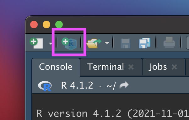
Let’s make an R Project so we can stay organized in the next steps.

Click the new R Project button at the top left of RStudio:

New R Project

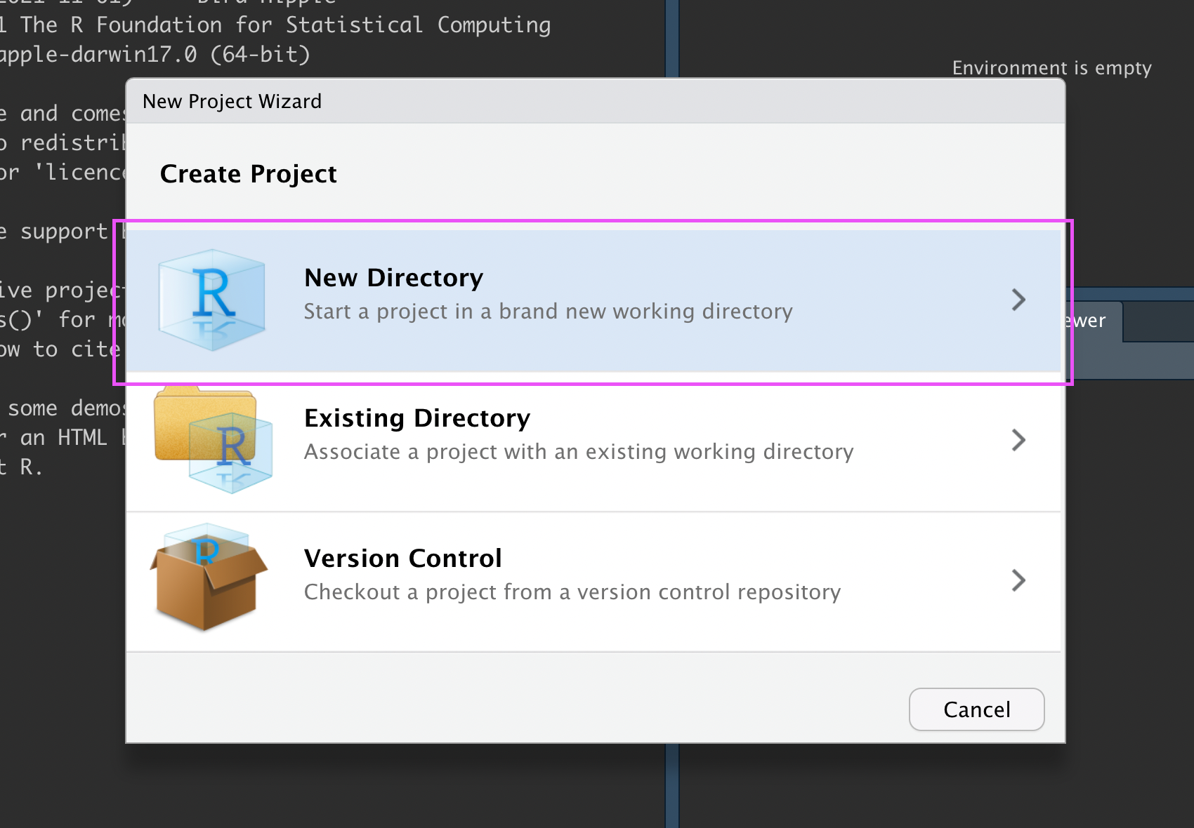
In the New Project Wizard, click “New Directory”:

New R Project

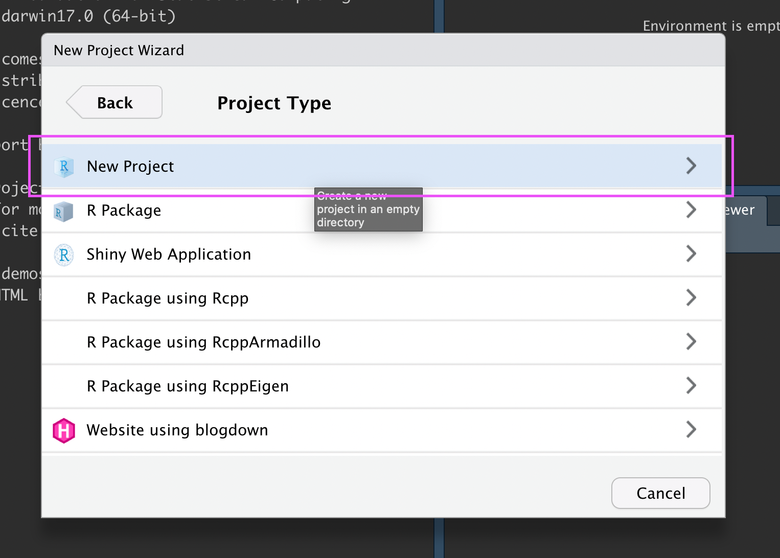
Click “New Project”:

New R Project

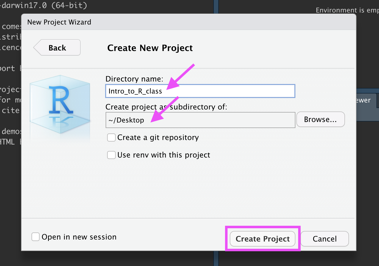
Type in a name for your new folder.

Store it somewhere easy to find, such as your Desktop:

New R Project

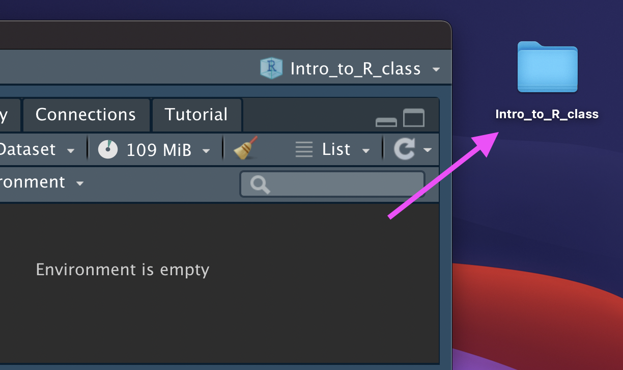
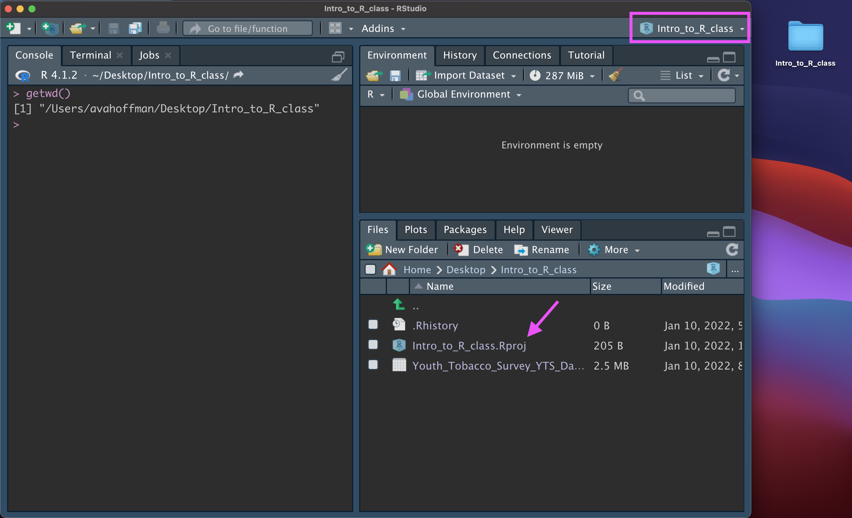
You now have a new R Project folder on your Desktop!

Make sure you add any scripts or data files to this folder as we go through today’s lesson. This will make sure R is able to “find” your files.

Data We Use

• Everything we do in class will be using real publicly available data
• Open Data and Data.gov will be sources for the first few days

Data Input

• ‘Reading in’ data is the first step of any real project/analysis
• R can read almost any file format, especially via add-on packages
• We are going to focus on simple delimited files first
  • comma separated (e.g. ‘.csv’)
  • tab delimited (e.g. ‘.txt’)
  • Microsoft Excel (e.g. ‘.xlsx’)

Data Input

Youth Tobacco Survey (YTS) dataset:

“The YTS was developed to provide states with comprehensive data on both middle school and high school students regarding tobacco use, exposure to environmental tobacco smoke, smoking cessation, school curriculum, minors’ ability to purchase or otherwise obtain tobacco products, knowledge and attitudes about tobacco, and familiarity with pro-tobacco and anti-tobacco media messages.”

• Check out the data at: https://catalog.data.gov/dataset/youth-tobacco-survey-yts-data

Data Input: Dataset Location

Dataset is located at https://github.com/chiraltraining/WW01_DataAnalysiswithR/blob/main/modules/07_Data_IO/YouthTobacco_newNames.csv

• Download data by clicking the above link

  • Google Chrome - if a file loads in your browser, choose File –> Save As, select, Format “Page Source” and save

Data Input: Read in Directly

# load library `readr` that contains function `read_csv`
library(readr)
dat <- read_csv("data/Youth_Tobacco_Survey_YTS_Data.csv")

# `head` displays first few rows of a data frame
head(dat, n = 5)

# A tibble: 5 × 31
   YEAR Locati…¹ Locat…² Topic…³ Topic…⁴ Measu…⁵ DataS…⁶ Respo…⁷ Data_…⁸ Data_…⁹
  <dbl> <chr>    <chr>   <chr>   <chr>   <chr>   <chr>   <chr>   <chr>   <chr>  
1  2015 AZ       Arizona Tobacc… Cessat… Percen… YTS     <NA>    %       Percen…
2  2015 AZ       Arizona Tobacc… Cessat… Percen… YTS     <NA>    %       Percen…
3  2015 AZ       Arizona Tobacc… Cessat… Percen… YTS     <NA>    %       Percen…
4  2015 AZ       Arizona Tobacc… Cessat… Quit A… YTS     <NA>    %       Percen…
5  2015 AZ       Arizona Tobacc… Cessat… Quit A… YTS     <NA>    %       Percen…
# … with 21 more variables: Data_Value <dbl>, Data_Value_Footnote_Symbol <chr>,
#   Data_Value_Footnote <chr>, Data_Value_Std_Err <dbl>,
#   Low_Confidence_Limit <dbl>, High_Confidence_Limit <dbl>, Sample_Size <dbl>,
#   Gender <chr>, Race <chr>, Age <chr>, Education <chr>, GeoLocation <chr>,
#   TopicTypeId <chr>, TopicId <chr>, MeasureId <chr>, StratificationID1 <chr>,
#   StratificationID2 <chr>, StratificationID3 <chr>, StratificationID4 <chr>,
#   SubMeasureID <chr>, DisplayOrder <dbl>, and abbreviated variable names …

Data Input: Read in Directly

So what is going on “behind the scenes”?

read_csv() parses a “flat” text file (.csv) and turns it into a tibble – a rectangular data frame, where data are split into rows and columns

• First, a flat file is parsed into a rectangular matrix of strings

• Second, the type of each column is determined (heuristic-based guess)

Data Input: Read in Directly

read_csv() needs the path to your file. It will return a tibble

read_csv(file, col_names = TRUE, col_types = NULL,
  locale = default_locale(), na = c("", "NA"),
  quoted_na = TRUE, quote = "\"", comment = "", trim_ws = TRUE,
  skip = 0, n_max = Inf, guess_max = min(1000, n_max),
  progress = show_progress(), skip_empty_rows = TRUE
)

• file is the path to your file, in quotes
• can be path in your local computer – absolute file path or relative file path
• can be path to a file on a website

## Examples

dat <- read_csv(file = "F:/VirtualWeekendWorkshops/VWW01_DataAnalysiswithR/modules/07_Data_IO/data")

dat <- read_csv(file = "Youth_Tobacco_Survey_YTS_Data.csv")

dat <- read_csv(file = "www.someurl.com/table1.csv")

Data Input: Read in Directly

Great, but what is my “path”?

Data Input: Read in Directly

Luckily, we already set up an R Project!

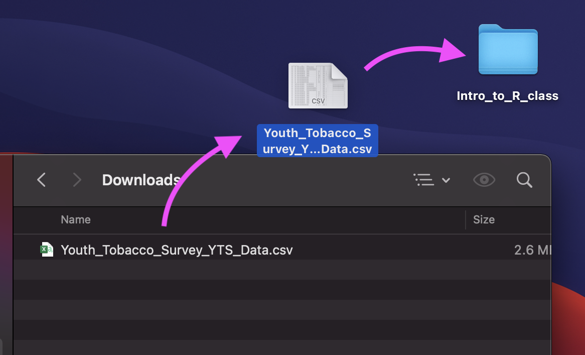
If we add the Youth_Tobacco_Survey_YTS_Data.csv file to the intro_to_r folder, we can use the relative path:

dat <- read_csv(file = "Youth_Tobacco_Survey_YTS_Data.csv")

Data Input: Read in Directly

read_csv() is a special case of read_delim() – a general function to read a delimited file into a data frame

read_delim() needs path to your file and file’s delimiter, will return a tibble

read_delim(file, delim, quote = "\"", escape_backslash = FALSE, 
  escape_double = TRUE, col_names = TRUE,  col_types = NULL, 
  locale = default_locale(),na = c("", "NA"),  quoted_na = TRUE, 
  comment = "", trim_ws = FALSE, skip = 0, 
  n_max = Inf,  guess_max = min(1000, n_max), 
  progress = show_progress(), skip_empty_rows = TRUE
)

• file is the path to your file, in quotes
• delim is what separates the fields within a record

## Examples
dat <- read_delim(file = "Youth_Tobacco_Survey_YTS_Data.csv", delim = ",")

dat <- read_delim(file = "www.someurl.com/table1.txt", delim = "\t")

Data Input: Read in Directly From File Path

dat <- read_csv(file = "data/Youth_Tobacco_Survey_YTS_Data.csv")

Rows: 9794 Columns: 31
── Column specification ────────────────────────────────────────────────────────
Delimiter: ","
chr (24): LocationAbbr, LocationDesc, TopicType, TopicDesc, MeasureDesc, Dat...
dbl  (7): YEAR, Data_Value, Data_Value_Std_Err, Low_Confidence_Limit, High_C...

ℹ Use `spec()` to retrieve the full column specification for this data.
ℹ Specify the column types or set `show_col_types = FALSE` to quiet this message.

The data is now successfully read into your R workspace. Column specification of first few columns is printed to the console.

Common new user mistakes we have seen

1. Working directory problems: trying to read files that R “can’t find”
   • Path misspecification
   • more on this shortly!
2. Typos (R is case sensitive, x and X are different)
   • RStudio helps with “tab completion”
3. Data type problems (is that a string or a number?)
4. Open ended quotes, parentheses, and brackets
   
5. Different versions of software

Data Input: Checking the data

• the View() function shows your data in a new tab, in spreadsheet format
• be careful if your data is big!

View(dat)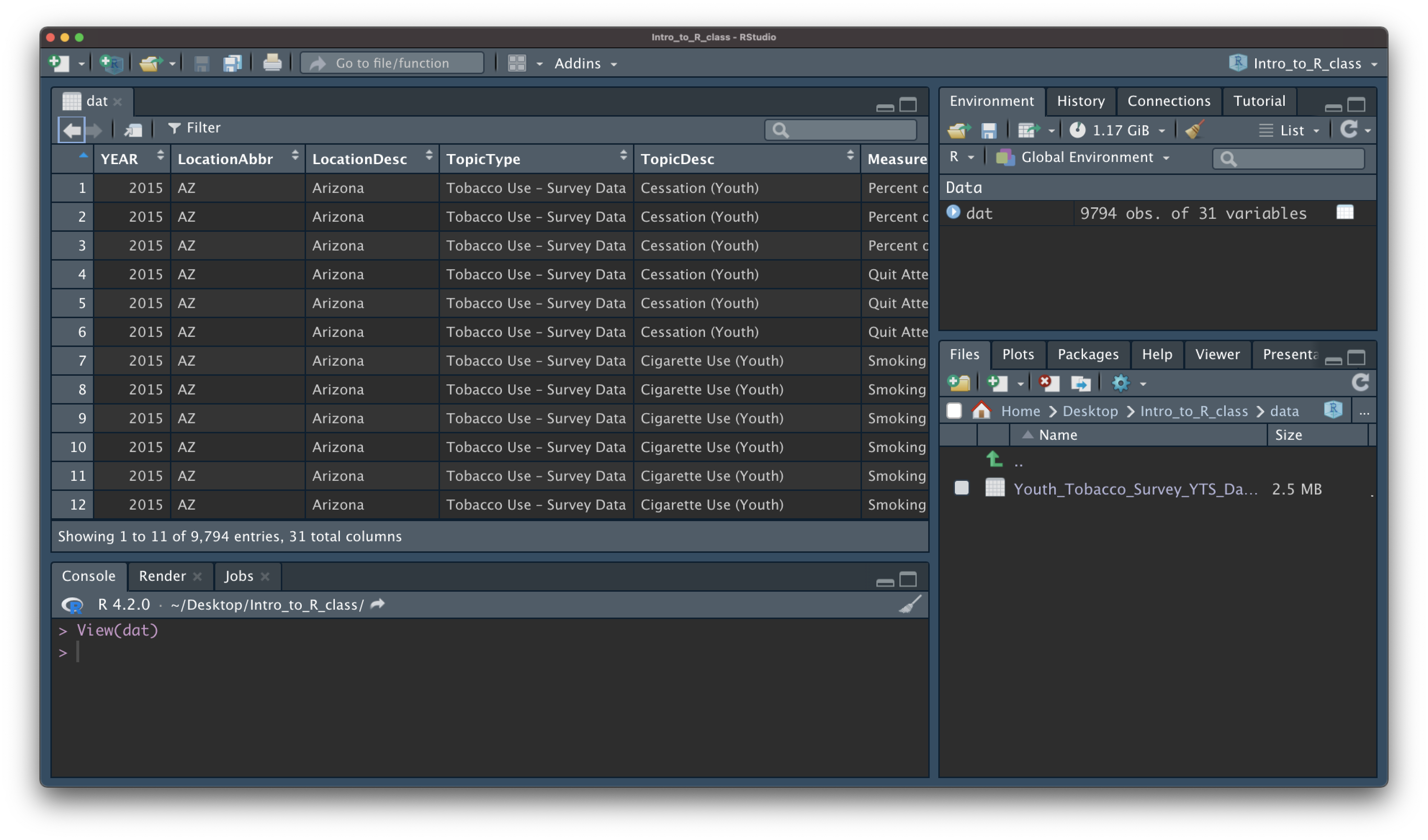

Data Input: Checking for problems

The spec() function shows you the specification of how the data was read in.

# dat <- read_csv("data/Youth_Tobacco_Survey_YTS_Data.csv")
spec(dat)

cols(
  YEAR = col_double(),
  LocationAbbr = col_character(),
  LocationDesc = col_character(),
  TopicType = col_character(),
  TopicDesc = col_character(),
  MeasureDesc = col_character(),
  DataSource = col_character(),
  Response = col_character(),
  Data_Value_Unit = col_character(),
  Data_Value_Type = col_character(),
  Data_Value = col_double(),
  Data_Value_Footnote_Symbol = col_character(),
  Data_Value_Footnote = col_character(),
  Data_Value_Std_Err = col_double(),
  Low_Confidence_Limit = col_double(),
  High_Confidence_Limit = col_double(),
  Sample_Size = col_double(),
  Gender = col_character(),
  Race = col_character(),
  Age = col_character(),
  Education = col_character(),
  GeoLocation = col_character(),
  TopicTypeId = col_character(),
  TopicId = col_character(),
  MeasureId = col_character(),
  StratificationID1 = col_character(),
  StratificationID2 = col_character(),
  StratificationID3 = col_character(),
  StratificationID4 = col_character(),
  SubMeasureID = col_character(),
  DisplayOrder = col_double()
)

Data Input: Checking for problems

The problems() function shows you if there were any obvious issues when the data was read in.

The output of problems() is a tibble showing each line with a concern.

problems(dat)

# A tibble: 0 × 5
# … with 5 variables: row <int>, col <int>, expected <chr>, actual <chr>,
#   file <chr>

Data Input: Checking for problems

dat looks good so far. What do you see on a messy dataset?

ufo_data <- read_csv(file = "https://github.com/SISBID/Data-Wrangling/blob/gh-pages/data/ufo/ufo_data_complete.csv")

problems(ufo_data)

# A tibble: 67 × 5
     row   col expected  actual      file 
   <int> <int> <chr>     <chr>       <chr>
 1    16   367 1 columns 367 columns ""   
 2    58     3 1 columns 3 columns   ""   
 3    79     3 1 columns 3 columns   ""   
 4   115     3 1 columns 3 columns   ""   
 5   123     6 1 columns 6 columns   ""   
 6   151     4 1 columns 4 columns   ""   
 7   161     4 1 columns 4 columns   ""   
 8   171     4 1 columns 4 columns   ""   
 9   181     4 1 columns 4 columns   ""   
10   191     4 1 columns 4 columns   ""   
# … with 57 more rows

Help

For any function, you can write ?FUNCTION_NAME, or help("FUNCTION_NAME") to look at the help file:

?read_delim
help("read_delim")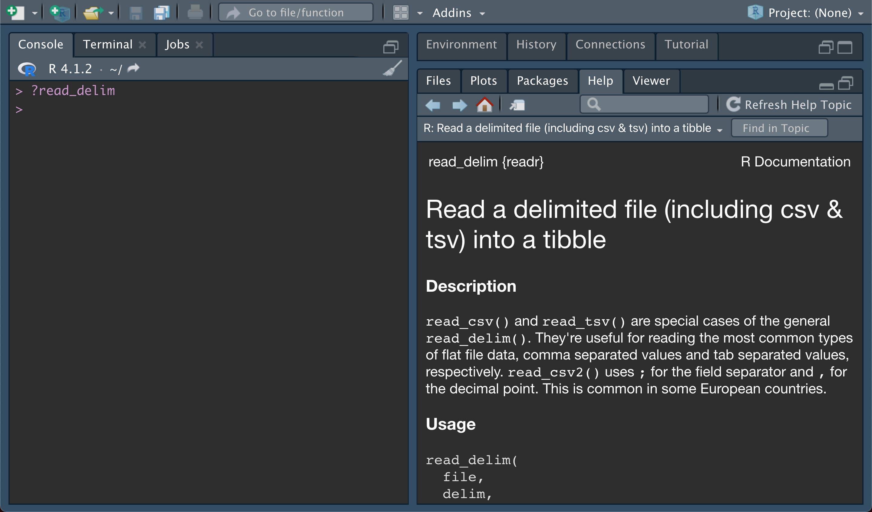

Data Input: Read in From RStudio Toolbar

R Studio features some nice “drop-down” support, where you can run some tasks by selecting them from the toolbar.

For example, you can easily import text datasets using the File --> Import Dataset --> From Text (readr) command. Selecting this will bring up a new screen that lets you specify the formatting of your text file.

After importing a dataset, the corresponding R command appears in the console.

Data Input: Read in From RStudio Toolbar

Data Input: base R

There are also data importing functions provided in base R (rather than the readr package), like read.delim() and read.csv().

These functions have slightly different syntax for reading in data (e.g. header argument).

However, while many online resources use the base R tools, the latest version of RStudio switched to use these new readr data import tools, so we will use them in the class for slides. They are also up to two times faster for reading in large datasets, and have a progress bar which is nice.

Data input: readr highlights

• Modern, improved tools from readr R package: read_delim(), read_csv()
  • needs a file path to be provided
  • parses the file into rows/columns, determines column type
  • returns a data frame
• Some functions to look at a data frame:
  • head() shows first few rows
  • tail() shows the last few rows
  • View() shows the data as a spreadsheet
  • spec() gives specification of column types

Data input: other file types

• From readr package:
  • read_delim(): general delimited files
  • read_csv(): comma separated (CSV) files
  • read_tsv(): tab separated files
  • others
• For reading Excel files, you can do one of:
  • use read_excel() function from readxl package
  • use other packages: xlsx, openxlsx

Data input: other file types

• haven package has functions to read SAS, SPSS, Stata formats

library(haven)

# SAS
read_sas(file = "mtcars.sas7bdat")

# SPSS
read_sav(file = "mtcars.sav")

# Stata
read_dta(file = "mtcars.dta")

Lab Part 1

💻 Data I/O Lab

Working Directories

Working directory is a directory that R assumes “you are working in”. It’s where R looks for files.

“Setting working directory” means specifying the path to the directory.

# get the working directory
getwd()

# set the working directory
setwd("/Users/avahoffman/Desktop")

R uses working directory as a starting place when searching for files.

Working Directories

R uses working directory as a starting place when searching for files:

• if you use read_csv("Bike_Lanes_Long.csv"), R assumes that the file is in the working directory

• if you use read_csv("data/Bike_Lanes_Long.csv"), R assumes that data directory is in the working directory

• if you use an absolute path, e.g. read_csv("/Users/avahoffman/data/Bike_Lanes_Long.csv"), the working directory information is not used

Working Directories

Setting up an R Project can avoid headaches by telling R that the working directory is wherever the .Rproj file is.

Data Output

While its nice to be able to read in a variety of data formats, it’s equally important to be able to output data somewhere.

The readr package provides data exporting functions which have the pattern write_*:

• write_csv(),
• write_delim(), others.

From write_csv() documentation:

write_csv(x, file, 
  na = "NA", append = FALSE, 
  col_names = !append, quote_escape = "double",
  eol = "\n", path = deprecated()
)

Data Output

x: data frame you want to write

file: file path where you want to R object written; it can be:

• an absolute path,
• a relative path (relative to your working directory),
• a file name only (which writes the file to your working directory)

# Examples

write_csv(dat, file = "YouthTobacco_newNames.csv")

write_delim(dat, file = "YouthTobacco_newNames.csv", delim = ",")

R binary file

.rds is an extension for R native file format.

write_rds() and read_rds() from readr package can be used to write/read a single R object to/from file.

Saving datasets in .rds format can save time if you have to read it back in later.

# write an object: a data frame "dat"
write_rds(dat, file = "yts_dataset.rds")

# write an object: vector "x"
x <- c(1, 3, 3)
write_rds(x, file = "my_vector.rds")

# read an object from file and assign to a new object named "y"
x2 <- read_rds(file = "my_vector.rds")
x2

[1] 1 3 3

Summary

• R Projects are a good way to keep your files organized and reduce headaches
• Use read_csv() and read_delim() from the readr package to read in your data
• Don’t forget to use <- to assign your data to an object!
• Use spec() to understand objects
• Use head() and tail() to preview the first and last lines of the data
• Use write_csv() and write_delim() from the readr package to write your (modified) data

🏠 Class Website

💻 Data I/O Lab